Lattices#
One day, I was sitting on a rooftop practicing some … breathing excercises … and it occured to me that maybe graft and prune form a lattice. I didn’t really know what a lattice was, so I went downstairs, pulled up the wikipedia definition and coded up some python to check which conditions were satisfied. It went pretty well.
It turns out there’s a whole family of different type of lattices that form a kind of poset themselves:
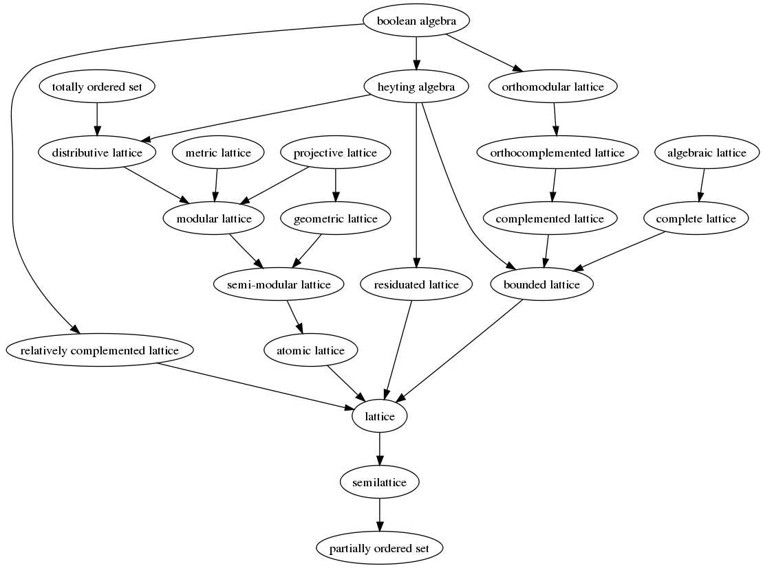
Almost immediately, I realized I had accidentally discovered a distributive lattice. A week later, I had proven it. The next week, I looked into connections with lattice based cryptography. Turns out to be a completely different lattice and massive waste of time. Just goes to show that not only do mathematicians suck at naming things, they can’t even do it uniquely. Anyway, after a few more months, I finally worked out how to produce Boolean algebras, right at the top. The following sections detail this journey but with hindsight’s gift of clarity.
Poset#
As you can see from the image above, a lattice is at the very least a partial order. So how do we make a productive partial order?
First of all, it makes sense to require that \(0\) is less than everything else:
I’ve chosen the \(\sqsubseteq\) symbol to maintain the square vibes.
The other natural requirements are for the primes to be incomparable and that if \(x \sqsubseteq y\), then \([x] \sqsubseteq [y]\). This second part generalizes to:
And that’s it. According to a pedantic redditor, we’ll also need the following which basically says \(0\) is definitely the smallest prod:
Let’s try a couple of examples:
\([] \sqsubseteq []\). Remember that \([] = [0]\) by (15). Since \(0 \sqsubseteq 0\) by (22), then \([0] \sqsubseteq [0]\) by (23).
\([] \sqsubseteq x\), for any \(x \neq 0\). Expand \([]\) to \([0, ..., 0]\) and \(x\) to \([x_1, ..., x_n]\). Apply (22) to every component and then (23) on the whole thing.
\([[]] \sqsubseteq [[], []]\). Firstly, pad \([[]]\) to \([[], 0]\). We just saw that \([] \sqsubseteq []\). Meanwhile, \(0 \sqsubseteq []\) by (22). So by (23), \([[], 0] \sqsubseteq [[], []]\).
\([[], 0] \not \sqsubseteq [0, []]\). \(0 \sqsubseteq []\) so both sides are part greater and part less than the other. Since neither is uniformly greater, we cannot use (23), so different primes are incomparable.
\([[[]]] \not \sqsubseteq [[0, []]]\). We just saw that \([[]] \not \sqsubseteq [0, []]\), so of course wrapping each side in another bracket doesn’t change anything. But this is example is important because the corresponding numbers divide: \(4 | 8\). Therefore \(\sqsubseteq\) is different to divisibility.
Here’s a snapshot of the Hasse diagram:

Once again, its much easier to interpret things with trees. The general pattern is that \(x \sqsubseteq y\) if you can place \(y\) on top of \(x\) and completely smother \(x\). Practice a few for yourself if you want.
Other than the \(4|8\) thing and the fact that the productive poset includes \(0\), hopefully you can see there’s a lot of similarities between the divisibility poset and the productive poset above. In fact, the productive poset is hidden inside the divisibility one!
Theorem 6
\(x \sqsubseteq y \implies x | y \text{, for any } x \neq 0\)
Proof - very insightful but involves some number theory
Remember that technically we are proving \(x \sqsubseteq y \implies I(x) | I(y)\) because the LHS is about prods and the RHS is about multiplicative numbers. For this proof only, I will revert to distinguishing \(x\) and \(I(x)\) because otherwise things can get a little confusing.
\(0\) needs to be excluded from the statement because \(0\) does not divide anything. But this means we can’t use induction on the main statement. Instead, we first prove it for \(\leq_+\), the total additive order from (10). This can be boosted to the divisibility order.
The proofs rely on the following facts:
If \(x \leq_+ y\), then \(p^x \leq_+ p^y\)
If \(x_1 \leq_+ y_1\) and \(x_2 \leq_+ y_2\) then \(x_1x_2 \leq_+ y_1y_2\)
\(p^x | p^y \iff x \leq_+ y\)
If \(x_1|y_1\) and \(x_2|y_2\) then \(x_1 x_2 | y_1 y_2\)
These all seem obvious to me. I refrain from proving them because I’m not a number theorist.
Lemma 2
\(x \sqsubseteq y \implies I(x) \leq_+ I(y)\)
Proof. Induction!
Base cases:
(\(x = 0\)): \(0 \leq_+ y\), for any \(y\) so that’s fine.
(\(y = 0\)): \(x \sqsubseteq 0\) means \(x = 0\) by (24), so that’s also fine.
Inductive step (\(x = [x_1, ..., x_n], y = [y_1, ..., y_n]\)): assume for inductive hypothesis that \(x_i \sqsubseteq y_i \implies I(x_i) \leq_+ I(y_i)\).
Assuming \(x \sqsubseteq y\), then \(x_i \sqsubseteq y_i\) by (23) and so \(I(x_i) \leq_+ I(y_i)\) by IH.
So from the first number theory assumption, \(p_i^{I(x_i)} \leq_+ p_i^{I(y_i)}\).
But from (17) \(I(x) = \prod_{i=1}^n p_i^{I(x_i)}\) and \(I(y) = \prod_{i=1}^n p_i^{I(x_i)}\). So just apply the second number theory assumption to get \(I(x) \leq_+ I(y)\).
That completes the first part. Proving it for the divisibility order is much easier.
Proof. (Proof of main theorem)
Since \(x \neq 0\) means \(y \neq 0\), expand \(x = [x_1, ..., x_n]\) and \(y = [y_1, ..., y_n]\).
\(x \sqsubseteq y\) means \(x_i \sqsubseteq y_i\) and so \(I(x_i) \leq_+ I(y_i)\) by the lemma. So by the third number theory fact, \(p_i^{I(x_i)} | p_i^{I(y_i)}\).
Applying the final number theory fact, \(I(x) = \prod_{i=1}^n p_i^{I(x_i)} | \prod_{i=1}^n p_i^{I(y_i)} = I(y)\)
Done.
Theorem 6 is subtle but possibly the most important conceptual result so far. While it makes sense to think of the productive order as a small deviation from the divisibility order, I think the proof highlights how the divisibility order is actually more closely related to the additive order. So maybe the visual similarities of the Hasse diagrams is because we’re just looking at the beginning parts and the higher you go, the sparser the similarities. Or maybe not. But it’s worth pondering.
In any case, we’d probably better check that \(\sqsubseteq\) really does define a partial order. I’ll go through the reflexivity proof in ‘’detail’’ and you can check out the other parts if you want. They’re all not-particularly-insightful inductions. Quick reminder in case you skipped the previous proofs: productive induction is just: prove it for \(0\), then assume it for \(x_1, ... x_n\) and prove it for \([x_1, ..., x_n]\).
Lemma 3
\(x \sqsubseteq x\)
Proof. Base case (\(x=0\)): \(0 \sqsubseteq 0\) by (22)
Inductive step (\(x = [x_1, ..., x_n]\)). Assume for inductive hypothesis \(x_i \sqsubseteq x_i\) for every \(i\). Then by (23), \([x_1, ..., x_n] \sqsubseteq [x_1, ..., x_n]\), so \(x \sqsubseteq x\). Done.
Click me for proofs of transitivity and anti-symmetry
We’ll go with anti-symmetry first because its merely a double induction.
Lemma 4
\(x \sqsubseteq y \land y \sqsubseteq x \implies x = y\)
Proof. Base cases: If \(x=0\) then \(y \sqsubseteq 0\), so \(y = 0 = x\) by (24). Similarly for \(y=0\).
Inductive step (\(x = [x_1, ..., x_n], y = [y_1, ..., y_n])\). As usual, we can assume \(x\) and \(y\) have the same length by padding. Assume for inductive hypothesis that \(x_i \sqsubseteq y_i \land y_i \sqsubseteq x_i \implies x_i = y_i\).
Since \(x \sqsubseteq y\), then \(x_i \sqsubseteq y_i\) for every \(i\) by (23). Similarly, \(y \sqsubseteq x\) implies \(y_i \sqsubseteq x_i\).
Now apply inductive hypothesis to get \(x_i = y_i\). So \([x_1, ..., x_n] = [y_1, ..., y_n]\) and \(x = y\). Done.
Transitivity triple induction time!
Lemma 5
\(x \sqsubseteq y \land y \sqsubseteq z \implies x \sqsubseteq z\)
Proof. Base case split on \(x,y,z\):
\(x=0\) immediately implies \(x \sqsubseteq z\) by (22).
\(y=0\) and \(x \sqsubseteq y\) implies \(x = 0\) by (24) and so \(x \sqsubseteq z\).
\(z=0\) and \(y \sqsubseteq z\) implies \(y=0\) which implies \(x=0\) (both by (24)) and so \(x \sqsubseteq z\).
Inductive step (\(x = [x_1, ..., x_n], y=[y_1, ..., y_n], z=[z_1, ..., z_n]\)): assume for inductive hypothesis that \(x_i \sqsubseteq y_i \land y_i \sqsubseteq z_i \implies x_i \sqsubseteq z_i\), for every \(i\).
Then \(x \sqsubseteq y\) implies \(x_i \sqsubseteq y_i\) by (23). Similarly, \(y \sqsubseteq z\) implies \(y_i \sqsubseteq z_i\).
Applying inductive hypothesis, \(x_i \sqsubseteq z_i\) for every \(i\). So \([x_1, ..., x_n] \sqsubseteq [z_1, ..., z_n]\) which means \(x \sqsubseteq z\) by (23). Done.
These proofs are so mechanical and uninteresting I don’t really see the point in reading them. Most of my intuition for \(\sqsubseteq\) comes from its semantic similarities to \(\subseteq\) and \(|\). But if that’s too informal for you, symbol shunt away!
Recall that trick I mentioned about fitting \(y\) on top of \(x\) to check whether its bigger. If you’ve read the wikipedia article on lattices closely (or just know enough about them already), you’ll know that there’s two different ways to define a lattice: either starting with a poset and looking for greatest/least upper/lower bounds or starting with two operations \(\land, \lor\) and using them to define a poset. Conveniently, these are identical in our case.
Theorem 7
\(x \sqsubseteq y \iff x = x \sqcap y\)
Click me for proof of equivalence
You’d never have guessed - its more inductions!
Proof. Forwards direction: \(x \sqsubseteq y \implies x = x \sqcap y\)
Base case (\(x = 0\)): \(0 \sqcap y = 0\) by (20).
Inductive step (\(x = [x_1, ..., x_n]\)): suppose \(x \sqsubseteq y\). Then \(y \neq 0\) by (24), so let \(y = [y_1, ..., y_n]\).
By (23), we have \(x_i \sqsubseteq y_i\). By inductive hypothesis, \(x_i = x_i \sqcap y_i\).
Therefore, \(x \sqcap y = [x_1, ..., x_n] \sqcap [y_1, ..., y_n] = [x_1 \sqcap y_1, ..., x_n \sqcap y_n] = [y_1, ..., y_n] = y\). Done.
Backwards direction: \(x = x \sqcap y \implies x \sqsubseteq y\).
Base case (\(x = 0\)): \(0 \sqsubseteq y\) by (22).
Inductive step (\(x = [x_1, ..., x_n]\)): suppose \(x = x \sqcap y\). Then \(y \neq 0\) by (24), so let \(y = [y_1, ..., y_n]\).
By (21), \(x_i = x_i \sqcap y_i\). By inductive hypothesis, \(x_i \sqsubseteq y_i\). Therefore, \(x \sqsubseteq y\) by (23). Done.
Historical Tangent
This equivalence was pretty exciting for me when I first noticed it because I had written down the definitions of \(\sqsubseteq\) and \(\sqcap\) completely independently, years apart, and they ended up working together in the nicest possible way, forming some structure I had barely even heard of. The only link between their definitions was that both times, I had tried to write down the simplest thing I could imagine. This gave the same sense of eery excitement you might get from realizing the way you butter your toast is the same as the way you brush your teeth, and these similiarities could help you solve a rubik’s cube.
The fact that both definitions had split into a \(0\) case and a \([x_1, ..., x_n]\) case is what led me to write down (13) and (14), where your journey began. Only then did I realize I could prove things by induction at which point the proofs wrote themselves and I could write this book. Coincidences like these are what convince me that prods (actually all math) are discovered, not invented.
So we’ve made it onto the first rung of the map!
Lattice#
To prove \(\sqcup, \sqcap\) form a lattice, we’ll continue ripping off the wikipedia definition. So we need:
Commutativity: \(x \sqcup y = y \sqcup x\) and \(x \sqcap y = y \sqcap x\)
Associativity: \((x \sqcup y) \sqcup z = x \sqcup (y \sqcup z)\) and \((x \sqcup y) \sqcup z = x \sqcup (y \sqcup z)\)
Absorption: \(x \sqcup (x \sqcap y) = x\) and \(x \sqcap (x \sqcup y) = x\)
I won’t prove all of these because the proofs are all dull, mechanical inductions. But here’s a couple for illustration.
Lemma 6
\(x \sqcup y = y \sqcup x\)
Proof. Base cases: clearly if either \(x\) or \(y\) is \(0\) then just use (18).
Inductive step (\(x = [x_1, ..., x_n], y = [y_1, ..., y_n]\)). Assume for inductive hypothesis that \(x_i \sqcup y_i = y_i \sqcup x_i\). Then \(x \sqcup y = [x_1 \sqcup y_1, ..., x_n \sqcup y_n] = [y_1 \sqcup x_1, ..., y_n \sqcup x_n] = y \sqcup x\). Done.
The only thing that would change for the proof of \(x \sqcap y = y \sqcap x\) would be the base cases, which still of course go through.
Lemma 7
\(x \sqcup (x \sqcap y) = x\)
Proof. Base cases:
(\(x = 0\)): \(0 \sqcup (0 \sqcap y) = 0 \sqcup 0 = 0\)
(\(y = 0\)): \(x \sqcup (x \sqcap 0) = x \sqcup x = x\), by Lemma 1
Inductive step (\(x = [x_1, ..., x_n], y = [y_1, ..., y_n]\)): assume for inductive hypothesis that \(x_i \sqcup (x_i \sqcap y_i) = x_i\), for every \(i\).
Then:
Done.
Obviously the proof of the other absorption law looks very similar, though you’d have to prove \(x \sqcap x = x\) first. I’m not going to bother with the associativity proofs because you either get the idea at this point, or you should stop reading and revisit some older chapters.
So we’ve hit lattice - the third rung! While we’re on a roll, we can jump way further to distributive lattice which you can see somewhere in the top left of the map. All we need is the following.
Theorem 8
\(x \sqcap (y \sqcup z) = (x \sqcap y) \sqcup (x \sqcap z)\)
Distributivity basically means that the two operations work smoothly with each other. Plug in \(\times, +\) and it should look more familiar.
Proof. Base cases:
(\(x=0\)): \(0 \sqcap (y \sqcup z) = 0 = 0 \sqcup 0 = (0 \sqcap y) \sqcup (0 \sqcap z)\)
(\(y=0\)): \(x \sqcap (0 \sqcup z) = x \sqcap z = 0 \sqcup (x \sqcap z) = (x \sqcap 0) \sqcup (x \sqcap z)\)
(\(z=0\)): follows from previous case by commutativity (Lemma 6)
Inductive step (\(x = [x_1, ..., x_n], y = [y_1, ..., y_n], z = [z_1, ..., z_n]\)): Assume for inductive hypothesis that \(x_i \sqcap (y_i \sqcup z_i) = (x_i \sqcap y_i) \sqcup (x_i \sqcap z_i)\).
Then:
Done.
Although that last one is yet another tedious induction, I remember finding it the most surprising and was possibly the first thing I properly proved about prods. So it holds quite a special place in my heart.
Heyting Algebra#
So we’ve got a distributive lattice. The next step up on the map is either totally ordered set (which we definitely don’t have) or something called a Heyting algebra. Apparently, a Heyting algebra means you can do logic inside a lattice which sounds pretty fun. You’ll notice that Heyting algebra is also above bounded lattice, so that’s a sort of pre-requisite for getting to Heyting.
In a bounded lattice, there’s a least element \(\bot\) that’s less than everything and a greatest element \(\top\) that’s bigger than everything. Clearly, \(0\) works for our least element. The greatest element is not so obvious. One option would be to artificially insert some element \(\top\) that just by definition is greater than everything, i.e. \(x \sqsubseteq \top\), for any \(x\) (which is equivalent to \(x \sqcap \top = x\) by Theorem 7).
This works to get a bounded lattice but, as punishment for the artificiality, can take us no further. Let’s have a look.
In a Heyting algebra, the idea is to interpret \(a \leq b\) as saying that \(a\) allows you to prove \(b\). So \(a \land b \leq a\) means that you can prove \(a\) from \(a\) and \(b\), which makes sense. \(\bot\) is interpreted as false and \(\top\) is interpreted as true, and everything else is a sort of intermediate truth value I don’t understand. The crucial requirement to be a Heyting algebra is that for every \(a,b\) there exists a greatest \(x\) such that \(a \land x \leq b\). This \(x\) is often called \(a \to b\) since \(a \land (a \to b) \leq b\), i.e. from \(a\) and \(a \to b\) you can prove \(b\). The fact that \(x\) is the greatest kind of means its the best at proving \(b\).
In the productive lattice, it’s easy to always find some \(x\) such \(a \sqcap x \sqsubseteq b\) - just choose \(x = 0\) since \(a \sqcap 0 = 0 \sqsubseteq b\), for any \(a,b\). The problem is finding the greatest \(x\). For example, imagine \(a = [0, []]\) and \(b = []\). Then \([[]]\) would work for \(x\) because \([0, []] \sqcap [[]] = [] \sqsubseteq []\). But so would \([[[]]]\) and \([[[[]]]]\), and so on forever up the \(2\) chain. On the other hand, picking \(\top\) doesn’t work because \([0, []] \sqcap \top = [0, []] \not \sqsubseteq []\). So there is no greatest \(x\), so we don’t have a Heyting algebra. Yet.
The problem is that the productive lattice is currently too large. So the obvious next step (which wasn’t obvious to me until a friend suggested it) is to try smaller lattices. Given a prod \(x\), we can take the set of prods smaller than it. Technically, this is called the downset of \(x\), written \(\downarrow x = \{y : y \sqsubseteq x \}\). Here’s the downset of \(30 = [[], [], []]\):

Note only does this look pretty (and very similar to this), but it forms a baby lattice of its own! This automatically makes it a Heyting algebra because its finite. We just have to prove a couple of things.
Theorem 9
For any \(x \in \mathbb{\Pi}, \downarrow x\) is a Heyting algebra.
Proof. Every finite distributive lattice is a Heyting algebra, so we’ll actually prove that instead. That \(\downarrow x\) is finite is obvious. Distributivity is inherited from the larger lattice. We just have to make sure that if \(y, z \in \downarrow x\), then \(y \sqcup z\) and \(y \sqcap z\) are both still in \(\downarrow x\). In other words, \(\sqcup\) and \(\sqcap\) cannot take you out of the downset.
Proving it for \(\sqcap\) is easy. It’s always the case that \(y \sqcap z \sqsubseteq y \sqsubseteq x\), so \(y \sqcap z \sqsubseteq x\) by transitivity.
For \(\sqcup\) we can use induction on the statement \(y,z \sqsubseteq x \implies y \sqcup z \sqsubseteq x\). There could be nicer ways but whatever.
Base cases:
if \(x=0\), then \(\downarrow x\) contains only \(0\) so there’s nothing to check.
if \(y=0\), then \(0 \sqcup z = z \sqsubseteq x\). Same for \(z = 0\).
Inductive step (\(x=[x_1, ..., x_n], y=[y_1, ..., y_n], z=[z_1,..., z_n]\)): assume for inductive hypothesis that \(y_i,z_i \sqsubseteq x_i \implies y_i \sqcup z_i \sqsubseteq x_i\) for every \(i\).
Assuming \(y,z \sqsubseteq x\), then \(y_i, z_i \sqsubseteq x_i\). So applying IH, \(y_i \sqcup z_i \sqsubseteq x_i\). Therefore, \(y \sqcup z = [y_1 \sqcup z_1, ..., y_n \sqcup z_n] \sqsubseteq [x_1, ..., x_n] = x\). Done.
Once you have \(a \to b\) for every element, you can define the opposite of \(a\) as \(a \to \bot\). This is usually written \(\lnot a\) (i.e. not \(a\)) because if \(a\) gives you a proof of false, then \(a\) had better be false!
If you choose \(0\) as \(\bot\), things don’t go very well: \(a \to 0\) will always be \(0\). On the other hand, if you get rid of \(0\) from your downsets, some nice structure appears. \(\bot\) becomes \([]\) and since there are more ways \(\sqcap\) can create \([]\), you get more interesting values for \(a \to []\). For example, in the \(30\) lattice from above (but without \(0\)), \(\lnot [[]] = [0, [], []]\). In general, you can kind of hop across the diagonal.
Getting rid of \(0\) is kind of ad-hoc. I’ve done it just to make the structure nicer. But interestingly it also makes the lattice closer to the divisibility one. So maybe there’s also good reasons.
Boolean Algebras#
Brief tangnet which I promise is relevant.
If the average science bro is to be believed, Logic gives you the sort objective rational access to Truth that in a different era was attributed to God. However, as you soon as you start studying formal logic you learn that there’s actually several different types of logics and (as with most things) their relative merits depend on the context in which you’re using them.
Two different logics which concern us here are classical vs. intuitionistic logic. Classical logic is the most popular and what people usually mean when they talk about Logic with a capital L. Classical logic is like the smug uncle who loves arguing with everyone at the Thanksgiving table. Intuitionistic logic (despite the terrible name) is like the shy cousin who knows better but only chimes in when they’re absolutely sure. The historical origin of intuitionism went something like this:
Formally speaking, the difference between the logics all comes down to whether or not you’re willing to automatically assume that for any \(a\), \(a \lor \lnot a\) (i.e. either \(a\) or not \(a\)). This is called the Law of Excluded Middle because it rules out any weird edge cases between True and False. Classical logicians say yes to excluded middle, intuitionistic logicians don’t. It’s worth emphasizing intuitionists don’t assume the opposite (though there is another logic which allows it), they just stay silent on it. While the classical logician says “of course \(a\) is either true of false”, the intuitionist says “I am yet to prove \(a\) or \(\lnot a\)”.
Having been through a non-classical logic phase myself, it was quite a fun coincidence that intutionism appeared to be making a come back in a completely independent number system. From what I understand, lattices are a useful way of comparing the differences between classical and intuitionistic logic. Heyting is a dead intuitionist and so Heyting algebras are all about intuitionistic logic. Boole is a dead classical logician and so Boolean algebras are all about classical logic.
In particular, a Boolean algebra is a Heyting algebra which also satisfies the equation \(a \lor \lnot a = \top\) for every \(a\). The subset lattice from here is actually a Boolean algebra. The negation of a subset is the subset that has all and only the elements the first one didn’t, so taking the union gives back the whole set.
Let’s check some examples on \(\downarrow 30\) from before. Remember that \(\top\) is \([[], [], []]\) and \(\bot\) is \([]\) because we got rid of \(0\).
Recall \([[]] \to [] = [0, [], []]\). Then \([[]] \sqcup [0, [], []] = [[], [], []]\). No middle!
\([[], []] \to [] = [0, 0, []]\). Then \([[], []] \sqcup [0, 0, []] = [[], [], []]\). Middle excluded!
\([] \to [] = [[], [], []]\). \([] \sqcup [[], [], []] = [[], [], []]\). Middle-free
And so on. It turns out that \(\downarrow 30\) actually is a Boolean algebra. On the other hand, check out \(\downarrow 24\) (remembering that \(24 = 2^3 \times 3\)):

Now things get more interesting. \([[]] \to [] = [0, []]\) but then \([[]] \sqcup [0, []] = [[], []] \neq [[0, []], []]\)! So \([[]] \sqcup \lnot [[]] \neq \top\). So it’s not Boolean. It turns out the example of \(30\) was quite special. The downset of \(x\) is only Boolean when \(x\) is shallow, i.e. all of the \(x_i\) are \([]\) or \(0\). It’s very similar to the subset case, because shallow prods basically are just sets of primes.
Theorem 10
\(x\) is shallow if and only if \(\downarrow x\) is a Boolean algebra
Proof. In the forwards direction, assume that \(x\) is shallow. Then identify \(x\) with the set of primes \(\{p_1, ..., p_k\}\) such that \(x_i = []\) (since \(x\) is shallow, all other \(x_j\) are \(0\)). Then every \(y \sqsubseteq x\) corresponds to a subset of \(\{p_1, ..., p_k\}\). Since the lattice of subsets is a Boolean algebra, so is the lattice \(\downarrow x\).
In the other direction, suppose that \(x = [x_1, ..., x_n]\) is not shallow. Assume \(x_1\) is strictly greater than \([]\) (there’ll always be some \(x_i\) like this but assuming its \(x_1\) just means there’s fewer … in the proof). Thus we have an increasing chain \([[]] \sqsubset [x_1] \sqsubseteq x\).
Consider \(\lnot [[]] = [[]] \to []\). By definition, \([[]] \sqcap \lnot [[]] = []\) and so \(\lnot [[]] = [0, y_2, ..., y_n]\) for some \(y_i\). But that means \([[]] \sqcup \lnot [[]] = [[], y_2, ..., y_n] \sqsubset [x_1, y_2, ..., y_n] \sqsubseteq x\). Therefore \([[]] \sqcup \lnot [[]] \neq x\), so \(\downarrow x\) is not a Boolean algebra.
Reassuringly, the same dichotomy happens in the divisibility lattice for numbers that are square-free (which I regrettably only learnt after struggling on this for ages). The lattices of shallow prods are identical to those of square-free numbers which are both basically identical to subset lattices. So all of the interesting differences are amongst Heyting algebras. If I understood them better, that’s where I would look next.
Fin#
That’s it. Theorem 10 gets us to the top of the map. Big respect for reading this far - it definitely got a bit hairy near the end.
Having completed wikipedia’s instruction manual for lattices, I don’t really know where else to go next. So I leave it up to you. See this section for some vague suggestions.
Thanks for reading :)